- 本文为365天深度学习训练营 中的学习记录博客
- 原作者:K同学啊
import tensorflow as tf

gpus = tf.config.list_physical_devices("GPU")

if gpus:
    tf.config.experimental.set_memory_growth(gpus[0], True)  #设置GPU显存用量按需使用
    tf.config.set_visible_devices([gpus[0]],"GPU")

# 打印显卡信息,确认GPU可用
print(gpus)
[]
import numpy as np
import matplotlib.pyplot as plt
# 支持中文
plt.rcParams['font.sans-serif'] = ['SimHei']  # 用来正常显示中文标签
plt.rcParams['axes.unicode_minus'] = False  # 用来正常显示负号

import os,PIL,pathlib

#隐藏警告
import warnings
warnings.filterwarnings('ignore')

data_dir = r"C:\Users\11054\Desktop\kLearning\t9_learning\data"
data_dir = pathlib.Path(data_dir)

image_count = len(list(data_dir.glob('*/*')))

print("图片总数为:",image_count)
图片总数为: 3400
batch_size = 64
img_height = 224
img_width  = 224
"""
关于image_dataset_from_directory()的详细介绍可以参考文章:https://mtyjkh.blog.csdn.net/article/details/117018789
"""
train_ds = tf.keras.preprocessing.image_dataset_from_directory(
    data_dir,
    validation_split=0.2,
    subset="training",
    seed=12,
    image_size=(img_height, img_width),
    batch_size=batch_size)

"""
关于image_dataset_from_directory()的详细介绍可以参考文章:https://mtyjkh.blog.csdn.net/article/details/117018789
"""
val_ds = tf.keras.preprocessing.image_dataset_from_directory(
    data_dir,
    validation_split=0.2,
    subset="validation",
    seed=12,
    image_size=(img_height, img_width),
    batch_size=batch_size)

class_names = train_ds.class_names
print(class_names)
Found 3400 files belonging to 2 classes.
Using 2720 files for training.
Found 3400 files belonging to 2 classes.
Using 680 files for validation.
['cat', 'dog']
for image_batch, labels_batch in train_ds:
    print(image_batch.shape)
    print(labels_batch.shape)
    break
(64, 224, 224, 3)
(64,)
AUTOTUNE = tf.data.AUTOTUNE

def preprocess_image(image,label):
    return (image/255.0,label)

# 归一化处理
train_ds = train_ds.map(preprocess_image, num_parallel_calls=AUTOTUNE)
val_ds   = val_ds.map(preprocess_image, num_parallel_calls=AUTOTUNE)

train_ds = train_ds.cache().shuffle(1000).prefetch(buffer_size=AUTOTUNE)
val_ds   = val_ds.cache().prefetch(buffer_size=AUTOTUNE)
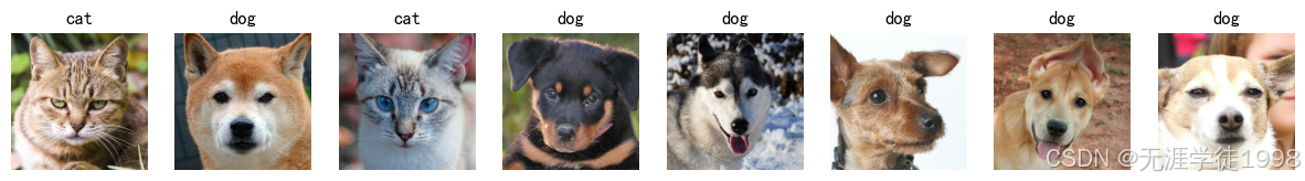
#可视化数据
plt.figure(figsize=(15, 10))  # 图形的宽为15高为10

for images, labels in train_ds.take(1):
    for i in range(8):

        ax = plt.subplot(5, 8, i + 1)
        plt.imshow(images[i])
        plt.title(class_names[labels[i]])

        plt.axis("off")
构建VGG-16
- VGG优缺点
- VGG优点
VGG的结构非常简洁,整个网络都使用了同样大小的卷积核尺寸(3x3)和最大池化尺寸(2x2) - VGG缺点
1)训练时间过长,调参难度大。2)需要的存储容量大,不利于部署。例如存储VGG-16权重值文件的大小为500多MB,不利于安装到嵌入式系统中
- 全连接层作用
- 主要作用是将输入的特征组合起来,以形成新的特征表示。在卷积神经网络(CNN)中,全连接层通常位于卷积层和池化层之后,用于将局部的特征组合成全局的特征表示。
- 通过在全连接层之后应用激活函数(如ReLU, Sigmoid, Tanh等),可以引入非线性变换,使模型能够拟合复杂的非线性关系。
- 全连接层包含大量的可训练参数(权重和偏置)。这些参数通过反向传播算法进行学习和优化,以最小化损失函数
- 分类问题中全连接层的输出通常会通过一个 Softmax 层(多分类)或 Sigmoid 层(二分类)转换成类别概率,从而完成最终的分类决策。
- 全连接层的每一个神经元与前一层的所有神经元相连接,将输入向量转换为输出向量,确保模型的输入和输出维度匹配。
from tensorflow.keras import layers, models, Input
from tensorflow.keras.models import Model
from tensorflow.keras.layers import Conv2D, MaxPooling2D, Dense, Flatten, Dropout

def VGG16(nb_classes, input_shape):
    input_tensor = Input(shape=input_shape)
    # 1st block
    x = Conv2D(64, (3,3), activation='relu', padding='same',name='block1_conv1')(input_tensor)
    x = Conv2D(64, (3,3), activation='relu', padding='same',name='block1_conv2')(x)
    x = MaxPooling2D((2,2), strides=(2,2), name = 'block1_pool')(x)
    # 2nd block
    x = Conv2D(128, (3,3), activation='relu', padding='same',name='block2_conv1')(x)
    x = Conv2D(128, (3,3), activation='relu', padding='same',name='block2_conv2')(x)
    x = MaxPooling2D((2,2), strides=(2,2), name = 'block2_pool')(x)
    # 3rd block
    x = Conv2D(256, (3,3), activation='relu', padding='same',name='block3_conv1')(x)
    x = Conv2D(256, (3,3), activation='relu', padding='same',name='block3_conv2')(x)
    x = Conv2D(256, (3,3), activation='relu', padding='same',name='block3_conv3')(x)
    x = MaxPooling2D((2,2), strides=(2,2), name = 'block3_pool')(x)
    # 4th block
    x = Conv2D(512, (3,3), activation='relu', padding='same',name='block4_conv1')(x)
    x = Conv2D(512, (3,3), activation='relu', padding='same',name='block4_conv2')(x)
    x = Conv2D(512, (3,3), activation='relu', padding='same',name='block4_conv3')(x)
    x = MaxPooling2D((2,2), strides=(2,2), name = 'block4_pool')(x)
    # 5th block
    x = Conv2D(512, (3,3), activation='relu', padding='same',name='block5_conv1')(x)
    x = Conv2D(512, (3,3), activation='relu', padding='same',name='block5_conv2')(x)
    x = Conv2D(512, (3,3), activation='relu', padding='same',name='block5_conv3')(x)
    x = MaxPooling2D((2,2), strides=(2,2), name = 'block5_pool')(x)
    # full connection
    x = Flatten()(x)
    x = Dense(4096, activation='relu',  name='fc1')(x)
    x = Dense(4096, activation='relu', name='fc2')(x)
    output_tensor = Dense(nb_classes, activation='softmax', name='predictions')(x)

    model = Model(input_tensor, output_tensor)
    return model

model=VGG16(1000, (img_width, img_height, 3))
model.summary()
Model: "functional"
┏━━━━━━━━━━━━━━━━━━━━━━━━━━━━━━━━━━━━━━┳━━━━━━━━━━━━━━━━━━━━━━━━━━━━━┳━━━━━━━━━━━━━━━━━┓
┃ Layer (type)                         ┃ Output Shape                ┃         Param # ┃
┡━━━━━━━━━━━━━━━━━━━━━━━━━━━━━━━━━━━━━━╇━━━━━━━━━━━━━━━━━━━━━━━━━━━━━╇━━━━━━━━━━━━━━━━━┩
│ input_layer (InputLayer)             │ (None, 224, 224, 3)         │               0 │
├──────────────────────────────────────┼─────────────────────────────┼─────────────────┤
│ block1_conv1 (Conv2D)                │ (None, 224, 224, 64)        │           1,792 │
├──────────────────────────────────────┼─────────────────────────────┼─────────────────┤
│ block1_conv2 (Conv2D)                │ (None, 224, 224, 64)        │          36,928 │
├──────────────────────────────────────┼─────────────────────────────┼─────────────────┤
│ block1_pool (MaxPooling2D)           │ (None, 112, 112, 64)        │               0 │
├──────────────────────────────────────┼─────────────────────────────┼─────────────────┤
│ block2_conv1 (Conv2D)                │ (None, 112, 112, 128)       │          73,856 │
├──────────────────────────────────────┼─────────────────────────────┼─────────────────┤
│ block2_conv2 (Conv2D)                │ (None, 112, 112, 128)       │         147,584 │
├──────────────────────────────────────┼─────────────────────────────┼─────────────────┤
│ block2_pool (MaxPooling2D)           │ (None, 56, 56, 128)         │               0 │
├──────────────────────────────────────┼─────────────────────────────┼─────────────────┤
│ block3_conv1 (Conv2D)                │ (None, 56, 56, 256)         │         295,168 │
├──────────────────────────────────────┼─────────────────────────────┼─────────────────┤
│ block3_conv2 (Conv2D)                │ (None, 56, 56, 256)         │         590,080 │
├──────────────────────────────────────┼─────────────────────────────┼─────────────────┤
│ block3_conv3 (Conv2D)                │ (None, 56, 56, 256)         │         590,080 │
├──────────────────────────────────────┼─────────────────────────────┼─────────────────┤
│ block3_pool (MaxPooling2D)           │ (None, 28, 28, 256)         │               0 │
├──────────────────────────────────────┼─────────────────────────────┼─────────────────┤
│ block4_conv1 (Conv2D)                │ (None, 28, 28, 512)         │       1,180,160 │
├──────────────────────────────────────┼─────────────────────────────┼─────────────────┤
│ block4_conv2 (Conv2D)                │ (None, 28, 28, 512)         │       2,359,808 │
├──────────────────────────────────────┼─────────────────────────────┼─────────────────┤
│ block4_conv3 (Conv2D)                │ (None, 28, 28, 512)         │       2,359,808 │
├──────────────────────────────────────┼─────────────────────────────┼─────────────────┤
│ block4_pool (MaxPooling2D)           │ (None, 14, 14, 512)         │               0 │
├──────────────────────────────────────┼─────────────────────────────┼─────────────────┤
│ block5_conv1 (Conv2D)                │ (None, 14, 14, 512)         │       2,359,808 │
├──────────────────────────────────────┼─────────────────────────────┼─────────────────┤
│ block5_conv2 (Conv2D)                │ (None, 14, 14, 512)         │       2,359,808 │
├──────────────────────────────────────┼─────────────────────────────┼─────────────────┤
│ block5_conv3 (Conv2D)                │ (None, 14, 14, 512)         │       2,359,808 │
├──────────────────────────────────────┼─────────────────────────────┼─────────────────┤
│ block5_pool (MaxPooling2D)           │ (None, 7, 7, 512)           │               0 │
├──────────────────────────────────────┼─────────────────────────────┼─────────────────┤
│ flatten (Flatten)                    │ (None, 25088)               │               0 │
├──────────────────────────────────────┼─────────────────────────────┼─────────────────┤
│ fc1 (Dense)                          │ (None, 4096)                │     102,764,544 │
├──────────────────────────────────────┼─────────────────────────────┼─────────────────┤
│ fc2 (Dense)                          │ (None, 4096)                │      16,781,312 │
├──────────────────────────────────────┼─────────────────────────────┼─────────────────┤
│ predictions (Dense)                  │ (None, 1000)                │       4,097,000 │
└──────────────────────────────────────┴─────────────────────────────┴─────────────────┘
Total params: 138,357,544 (527.79 MB)
Trainable params: 138,357,544 (527.79 MB)
Non-trainable params: 0 (0.00 B)
# 模型编译与运行
initial_learning_rate = 0.01
lr_schedule = tf.keras.optimizers.schedules.ExponentialDecay(
    initial_learning_rate,
    decay_steps=100000,
    decay_rate=0.92,
    staircase=True)
optimizer = tf.keras.optimizers.Adam(learning_rate=lr_schedule)
model.compile(optimizer=optimizer,
              loss     ='sparse_categorical_crossentropy',
              metrics  =['accuracy'])
from tqdm import tqdm
import tensorflow.keras.backend as K

epochs = 10
lr     = 1e-4

# 记录训练数据,方便后面的分析
history_train_loss     = []
history_train_accuracy = []
history_val_loss       = []
history_val_accuracy   = []

for epoch in range(epochs):
    train_total = len(train_ds)
    val_total   = len(val_ds)

    """
    total:预期的迭代数目
    ncols:控制进度条宽度
    mininterval:进度更新最小间隔,以秒为单位(默认值:0.1)
    """
    with tqdm(total=train_total, desc=f'Epoch {epoch + 1}/{epochs}',mininterval=1,ncols=100) as pbar:
        train_loss     = []
        train_accuracy = []
        for image,label in train_ds:
            """
            训练模型,简单理解train_on_batch就是:它是比model.fit()更高级的一个用法

            想详细了解 train_on_batch 的同学,
            可以看看我的这篇文章:https://www.yuque.com/mingtian-fkmxf/hv4lcq/ztt4gy
            """
             # 这里生成的是每一个batch的acc与loss
            history = model.train_on_batch(image,label)

            train_loss.append(history[0])
            train_accuracy.append(history[1])

            pbar.set_postfix({"train_loss": "%.4f"%history[0],
                              "train_acc":"%.4f"%history[1],
                              "lr": optimizer.learning_rate.numpy()})
            pbar.update(1)

        history_train_loss.append(np.mean(train_loss))
        history_train_accuracy.append(np.mean(train_accuracy))

    print('开始验证!')

    with tqdm(total=val_total, desc=f'Epoch {epoch + 1}/{epochs}',mininterval=0.3,ncols=100) as pbar:

        val_loss     = []
        val_accuracy = []
        for image,label in val_ds:
            # 这里生成的是每一个batch的acc与loss
            history = model.test_on_batch(image,label)

            val_loss.append(history[0])
            val_accuracy.append(history[1])

            pbar.set_postfix({"val_loss": "%.4f"%history[0],
                              "val_acc":"%.4f"%history[1]})
            pbar.update(1)
        history_val_loss.append(np.mean(val_loss))
        history_val_accuracy.append(np.mean(val_accuracy))

    print('结束验证!')
    print("验证loss为:%.4f"%np.mean(val_loss))
    print("验证准确率为:%.4f"%np.mean(val_accuracy))
Epoch 1/10:   7%| | 3/43 [00:58<12:50, 19.26s/it, train_loss=817908992.0000, train_acc=0.4844, lr=0.

WARNING:tensorflow:5 out of the last 5 calls to <function TensorFlowTrainer.make_train_function.<locals>.one_step_on_iterator at 0x0000026D58AB2670> triggered tf.function retracing. Tracing is expensive and the excessive number of tracings could be due to (1) creating @tf.function repeatedly in a loop, (2) passing tensors with different shapes, (3) passing Python objects instead of tensors. For (1), please define your @tf.function outside of the loop. For (2), @tf.function has reduce_retracing=True option that can avoid unnecessary retracing. For (3), please refer to https://www.tensorflow.org/guide/function#controlling_retracing and https://www.tensorflow.org/api_docs/python/tf/function for  more details.


Epoch 1/10:   9%| | 4/43 [01:17<12:21, 19.02s/it, train_loss=33623308288.0000, train_acc=0.4844, lr=

WARNING:tensorflow:6 out of the last 6 calls to <function TensorFlowTrainer.make_train_function.<locals>.one_step_on_iterator at 0x0000026D58AB2670> triggered tf.function retracing. Tracing is expensive and the excessive number of tracings could be due to (1) creating @tf.function repeatedly in a loop, (2) passing tensors with different shapes, (3) passing Python objects instead of tensors. For (1), please define your @tf.function outside of the loop. For (2), @tf.function has reduce_retracing=True option that can avoid unnecessary retracing. For (3), please refer to https://www.tensorflow.org/guide/function#controlling_retracing and https://www.tensorflow.org/api_docs/python/tf/function for  more details.


Epoch 1/10: 100%|█| 43/43 [13:22<00:00, 18.66s/it, train_loss=3165756416.0000, train_acc=0.4989, lr=


开始验证!


Epoch 1/10:  36%|███▋      | 4/11 [00:19<00:34,  4.88s/it, val_loss=2893433856.0000, val_acc=0.4940]

WARNING:tensorflow:5 out of the last 5 calls to <function TensorFlowTrainer.make_test_function.<locals>.one_step_on_iterator at 0x0000026DDF2E49D0> triggered tf.function retracing. Tracing is expensive and the excessive number of tracings could be due to (1) creating @tf.function repeatedly in a loop, (2) passing tensors with different shapes, (3) passing Python objects instead of tensors. For (1), please define your @tf.function outside of the loop. For (2), @tf.function has reduce_retracing=True option that can avoid unnecessary retracing. For (3), please refer to https://www.tensorflow.org/guide/function#controlling_retracing and https://www.tensorflow.org/api_docs/python/tf/function for  more details.


Epoch 1/10:  45%|████▌     | 5/11 [00:24<00:29,  4.87s/it, val_loss=2832519680.0000, val_acc=0.4951]

WARNING:tensorflow:6 out of the last 6 calls to <function TensorFlowTrainer.make_test_function.<locals>.one_step_on_iterator at 0x0000026DDF2E49D0> triggered tf.function retracing. Tracing is expensive and the excessive number of tracings could be due to (1) creating @tf.function repeatedly in a loop, (2) passing tensors with different shapes, (3) passing Python objects instead of tensors. For (1), please define your @tf.function outside of the loop. For (2), @tf.function has reduce_retracing=True option that can avoid unnecessary retracing. For (3), please refer to https://www.tensorflow.org/guide/function#controlling_retracing and https://www.tensorflow.org/api_docs/python/tf/function for  more details.


Epoch 1/10: 100%|█████████| 11/11 [00:51<00:00,  4.70s/it, val_loss=2532606720.0000, val_acc=0.4974]


结束验证!
验证loss为:2787614720.0000
验证准确率为:0.4958


Epoch 2/10: 100%|█| 43/43 [13:03<00:00, 18.23s/it, train_loss=1423662976.0000, train_acc=0.5020, lr=


开始验证!


Epoch 2/10: 100%|█████████| 11/11 [00:52<00:00,  4.74s/it, val_loss=1281297920.0000, val_acc=0.5026]


结束验证!
验证loss为:1341318784.0000
验证准确率为:0.5034


Epoch 3/10: 100%|█| 43/43 [13:02<00:00, 18.19s/it, train_loss=915221888.0000, train_acc=0.5022, lr=0


开始验证!


Epoch 3/10: 100%|██████████| 11/11 [00:52<00:00,  4.75s/it, val_loss=854207104.0000, val_acc=0.5026]


结束验证!
验证loss为:880286656.0000
验证准确率为:0.5031


Epoch 4/10: 100%|█| 43/43 [13:04<00:00, 18.24s/it, train_loss=674374464.0000, train_acc=0.5006, lr=0


开始验证!


Epoch 4/10: 100%|██████████| 11/11 [00:51<00:00,  4.71s/it, val_loss=640655744.0000, val_acc=0.5001]


结束验证!
验证loss为:655163968.0000
验证准确率为:0.4998


Epoch 5/10: 100%|█| 43/43 [13:01<00:00, 18.18s/it, train_loss=533879808.0000, train_acc=0.5004, lr=0


开始验证!


Epoch 5/10: 100%|██████████| 11/11 [00:52<00:00,  4.76s/it, val_loss=512524608.0000, val_acc=0.5007]


结束验证!
验证loss为:521749024.0000
验证准确率为:0.5010


Epoch 6/10: 100%|█| 43/43 [13:05<00:00, 18.28s/it, train_loss=441831552.0000, train_acc=0.4995, lr=0


开始验证!


Epoch 6/10: 100%|██████████| 11/11 [00:52<00:00,  4.75s/it, val_loss=427103840.0000, val_acc=0.4992]


结束验证!
验证loss为:433481824.0000
验证准确率为:0.4990


Epoch 7/10: 100%|█| 43/43 [13:07<00:00, 18.30s/it, train_loss=376856320.0000, train_acc=0.5020, lr=0


开始验证!


Epoch 7/10: 100%|██████████| 11/11 [00:51<00:00,  4.69s/it, val_loss=366089024.0000, val_acc=0.5022]


结束验证!
验证loss为:370760384.0000
验证准确率为:0.5024


Epoch 8/10: 100%|█| 43/43 [13:00<00:00, 18.16s/it, train_loss=328541408.0000, train_acc=0.5014, lr=0


开始验证!


Epoch 8/10: 100%|██████████| 11/11 [00:52<00:00,  4.74s/it, val_loss=320327872.0000, val_acc=0.5015]


结束验证!
验证loss为:323896160.0000
验证准确率为:0.5017


Epoch 9/10: 100%|█| 43/43 [13:07<00:00, 18.30s/it, train_loss=291207168.0000, train_acc=0.5030, lr=0


开始验证!


Epoch 9/10: 100%|██████████| 11/11 [00:52<00:00,  4.74s/it, val_loss=284735904.0000, val_acc=0.5027]


结束验证!
验证loss为:287550240.0000
验证准确率为:0.5026


Epoch 10/10: 100%|█| 43/43 [13:03<00:00, 18.21s/it, train_loss=261492144.0000, train_acc=0.5038, lr=


开始验证!


Epoch 10/10: 100%|█████████| 11/11 [00:52<00:00,  4.75s/it, val_loss=256262304.0000, val_acc=0.5039]

结束验证!
验证loss为:258538656.0000
验证准确率为:0.5041
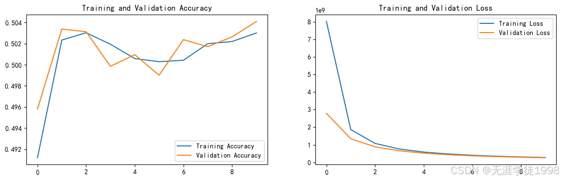
# 模型评估
epochs_range = range(epochs)

plt.figure(figsize=(14, 4))
plt.subplot(1, 2, 1)

plt.plot(epochs_range, history_train_accuracy, label='Training Accuracy')
plt.plot(epochs_range, history_val_accuracy, label='Validation Accuracy')
plt.legend(loc='lower right')
plt.title('Training and Validation Accuracy')

plt.subplot(1, 2, 2)
plt.plot(epochs_range, history_train_loss, label='Training Loss')
plt.plot(epochs_range, history_val_loss, label='Validation Loss')
plt.legend(loc='upper right')
plt.title('Training and Validation Loss')
plt.show()
个人总结
- K.set_value TensorFlow 2.16中已被弃用 可通过tf.keras.optimizers.schedules.ExponentialDecay设置动态学习率
- K.get_value TensorFlow 2.16中已被弃用 可通过current_lr = optimizer.learning_rate.numpy()获取当前学习率
本站资源均来自互联网,仅供研究学习,禁止违法使用和商用,产生法律纠纷本站概不负责!如果侵犯了您的权益请与我们联系!
转载请注明出处: 免费源码网-免费的源码资源网站 » T9打卡学习笔记

发表评论 取消回复